5 Estimation risk reduction techniques
As stated in chapter 3, estimation risk is comprised of squared bias and variance. There are many methods to approach reducing estimation risk, but in this research, we introduce three ways that are consistent with the general risk-based investing framework presented in equation (3.7). The first method deals with improving the estimation of the inputs to the risk-based portfolio function \(f(w, \Sigma|\textbf{X})\), accounting for heterogeneity in the input data. The second method involves penalising the optimisation objective function to obtain a portfolio estimate with consistently lower deviation from the actual out-of-sample risk-based portfolio solution. The final process entails changing the implementation method in a manner that reduces estimation risk. Every risk reduction technique falls into one of these three categories.
5.1 Improving optimisation inputs
The first approach to improving on the sample ERC and GMV portfolios involves finding better estimates for the input \(\Sigma\), given the set of sample returns. As stated in equation (3.5), the function \(g\) deals with the sample returns in a manner that ensures the irreducible error, \(\phi^2\), is independent and identically normally distributed. However, because \(g\) is unobservable, our estimation \(\hat{g}\) might not ensure this property. Heterogeneity of sample errors for investment portfolios has been observed in empirical finance by Ang and Chen (2002), who demonstrate that negative stock price correlations are less pronounced in downward markets. Therefore, empirical finance suggests two states of the world, one where the market is in turmoil, and one where the market is not.
Kritzman, Page, and Turkington (2012) use these two states to determine separate multi-asset allocations for ‘turbulent’ and ‘quiet’ markets and adopt a regime switching (RS) approach. To define two regimes, a metric to measure turbulence is required. The authors take a squared Mahalanobis distance (SMD) approach to determine an index through time. The Mahalanobis distance is a multi-dimensional generalisation of the notion of how many standard deviations a point is away from the mean of a distribution. The SMD index (\(d_t\)) is expressed mathematically as: \[\begin{align} d_t = (R_t - \mu)\Sigma^{-1}(R_t - \mu)^\intercal, \end{align}\] where: \[d_t = \mu_{s_t} + \sigma_{s_t}\epsilon_t,\] and \(\epsilon_t\) has a standard normal distribution. The state at time \(t\) is shown by the random variable \(s_t\). As asserted earlier, the two states are Quiet (\(Q\)) and Turbulent (\(T\)), hence \(s_t \in \{Q, T\}\). To calculate the SMD, we require the unobservable inputs \(\Sigma\) and \(\mu\). They can be replaced by their sample counterparts, \(\textbf{S}\) and \(\hat{\mu}\), to yield \(\hat{d}_t\). The SMD has a state-specific mean and volatility; hence different values are observed based on the current system state. If the system emits large values of \(\hat{d}_t\), the probability of being in a turbulent market is high. If the system emits small values of \(\hat{d}_t\), the likelihood of being in a quiet market is high. The \(\zeta^{th}\) quantile of the sample SMDs is the point where the system of reference changes. The market state is also an unobservable variable, so the above model is referred to as a hidden Markov model (HMM). The HMM used in this investigation is depicted in figure 5.1.
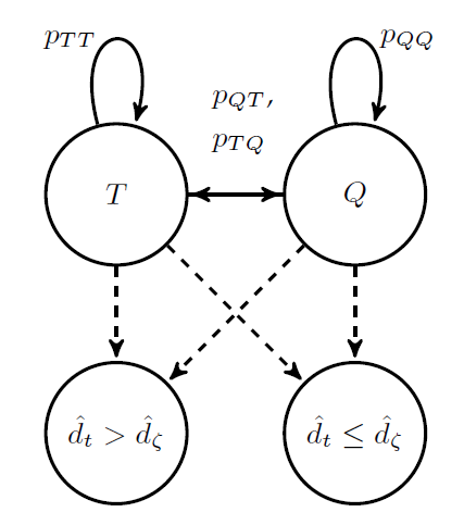
Figure 5.1: Turbulent / quiet hidden Markov model.
The transition matrix stores the probabilities of transition from a state at time \(t\) to another at time \(t + 1\) for ease of computation. It is mathematically shown as: \[P_{t, t + 1} = \begin{bmatrix} p_{QQ} & p_{QT} \\ p_{TQ} & p_{TT} \end{bmatrix},\] where the matrix applies to all times \(t\). Because the matrix applies to all times the system is called stationary, and the long-run probabilities of being in each state will converge. Once we have determined the most likely state at time \(t\) using an algorithm such as the Viterbi algorithm, we can use the series of estimated states \(\{\hat{s}_t: t \in \{0, 1, ..., T\}\}\) to partition the data history. The two datasets would be data used for the quiet sample covariance matrix and data used for the turbulent sample covariance matrix. Flint and Du Plooy (2018) blend these two sample matrices using the investor’s risk preferences and the most recent probabilities of being in each state, yielding a more sophisticated estimator of \(\Sigma\).
An alternative approach to dealing with heterogeneity is to focus on the assumption that errors for return forecasting models have a normal distribution. But first, we need to define a general return forecasting model. If the return of a portfolio is viewed through a set of return drivers or risk factors, then returns could be explained in part by those factors and the portfolio’s sensitivity to them. Meucci (2010) encapsulates this idea in his asset return model given below: \[\begin{align} R &= \alpha +\beta^\intercal \mathcal{F} + \epsilon, \tag{5.1} \end{align}\] where \(R\) is a vector of asset returns (not portfolio returns through time as shown previously), \(\alpha\) is a forecastable vector of returns unique to each security, \(\beta\) is a matrix of sensitivities to risk factors, \(\mathcal{F}\) is a vector of factors, and \(\epsilon\) is the error vector. The error vector is assumed to have a normal distribution. Ang and Chen (2002) show that in a downward market, the correlation structure is significantly different from what is implied by a normal distribution, which is a problem when using model (5.1) in the exhibited way. Chen, Dolado, and Gonzalo (2019) address the issue of non-normal errors by utilising the quantile regression model proposed by Koenker and Bassett Jr (1978). The asset returns, idiosyncratic asset returns, asset factor sensitivities and errors could all be considered to be a function of the current quantile, denoted \(\tau\). This leads to the quantile factor model (QFM): \[\begin{align} \mathcal{Q}(\tau) = \alpha(\tau) + \beta(\tau)\mathcal{F} + \epsilon(\tau), \tag{5.2} \end{align}\] where \(\tau \in [0, 1]\). In a different symmetric, normally distributed world, \(\tau\) can be set to \(0.5\) and model (5.1) will be recovered. However, in the real world where symmetry and normality are often not adhered to, the quantile conditional errors can be defined more generally so that they only have to satisfy: \[\begin{align} \mathbb{P}\Big[\epsilon(\tau) \leq \underline{0} \, \Big | \mathcal{F} \Big] = \tau \; . \end{align}\] This structure emerges from the cumulative distribution function (CDF) conditional on the set of factors of each asset return \(R_i\). Given the conditional CDF for the returns on asset \(i\), \(F_i(R_i|\mathcal{F})\), the quantile specific inverse CDF, \(F^{-1}_i(\tau| \mathcal{F})\), can be used to generate the quantiles \(\mathcal{Q}_i(\tau)\). Flint and Du Plooy (2018) suggest using the information about each quantile to construct a series of quantile-specific covariance matrices, which can then be blended to yield a more sophisticated estimator of \(\Sigma\). Chapter insert ref to next chapter covers the implementations of these two techniques to better estimate \(\Sigma\).
5.2 Penalising the optimization
To add a penalty term in a way that preserves the goal of the risk optimisation, we first need to adapt the objective functions of each risk-based portfolio as given earlier in chapter @ref{rbportch}. Consider the return-targeting penalised optimisation approach of Kinn (2018), both choices of \(f(\cdot|\textbf{X})\) for the GMV and ERC portfolios can be adapted into this approach. Beginning with the GMV portfolio, Kinn views the portfolio variance as an expectation: \[\begin{align*} f(w, \Sigma | \textbf{X}) &= w^\intercal \Sigma w &\\ & = w^\intercal (\mathbb{E}[{r}_t {r}_t^\intercal] - \mu \mu^\intercal) w & \small\text{(alternate definition of $\Sigma$)} \\ & = \mathbb{E}[|w^\intercal \mu - w^\intercal {r}_t|^2], \end{align*}\] where \({r}_t\) represents the asset returns above the risk-free rate, and \(\mu\) is a vector of the population expected excess returns as before. Rewriting the portfolio expected excess return as \(\bar{r} = w^\intercal \mu\), the idea of return-targeting for a portfolio can be incorporated as the expectation of \(|\bar{r} - w^\intercal {r}_t|^2\), which is the squared distance to a target return level. Kinn’s approach is consistent with an MVO optimisation intuitively because the target return level is analogous an expected return constraint and minimising the return’s squared distance to this constraint is analogous to variance minimisation. The objective function can now be approximated using the sample average as a result of the law of large numbers. We still have to show how to find the GMV portfolio from an MVO procedure. As stated in table 4.1, the GMV portfolio is the MSR portfolio if the assumption of identical excess returns is met. Therefore, if the target return is set to a value that is easily obtainable \(\bar{r} = \bar{r}_\mathrm{gmv}\), then the scheme will yield a GMV portfolio. This easily obtainable value has to be found numerically and cannot be determined a priori. The non-rigorous argument turns out to be empirically true for the portfolios analysed in this research. When the return vector is replaced by the set of sample returns \(\textbf{X}\), and the expectation is approximated by the sample average, the Kinn (2018) form of objective function is recovered: \[\begin{align} f_{\text{Kinn}}(w|\textbf{X}) &= \frac{1}{T} \sum_{t = 1}^T (\bar{r}_\mathrm{gmv} - \textbf{X}^\intercal_t w)^2, \tag{5.3} \end{align}\] where \(t\) indexes columns of the sample returns matrix \(\textbf{X}\). The GMV portfolio can be found equivalently in this way.
The log-constraint4, \(\sum_i \ln(w_i) \geq c\), can be placed on optimisation (5.3) to recover the ERC portfolio. To include the constraint in framework (3.7), a Lagrangian multiplier approach can be used to move the log-constraint to the objective function. Kinn’s adapted ERC objective function is then: \[\begin{align} f_{\text{Kinn}}(w|\textbf{X}) &= \frac{1}{T} \sum_{t = 1}^T (\bar{r}_{gmv} - \textbf{X}^\intercal_t w)^2 -\eta_{erc}\sum_{i = 1}^N \ln(w_i), \end{align}\] where \(\eta_{erc}\) is the Lagrangian multiplier scalar. Now that we have shown the standard objective functions from earlier are equivalent to the Kinn framework, we have also vindicated the general framework (3.7) as accommodative of a valid application of supervised machine learning (SML) to portfolio optimisation.
Because logical choices for \(f_{\text{Kinn}}(\cdot|\textbf{X})\) have been established, different penalty functions can be applied to the optimisation. Two common penalised regression techniques are lasso regression and ridge regression (RR). In the presence of a long-only constraint, as is applied in this research, a lasso regression does not make sense, because the penalty function is simply the sum of the absolute weights: \(P(w) = \sum_{i= 1}^N |w_i| =1\). This penalty is equal to \(1\) for all constrained portfolios. Separately, the RR is obtained by specifying the penalty as the sum of squares for the portfolio weights: \(P(w) = \sum_{i= 1}^N w_i^2\). The penalty reduces the number of admissable concentrated portfolios and intuitively is not unlike incorporating some of the EW portfolio into the ERC or GMV portfolios. Ignoring constraints, Ledoit and Wolf (2004) show that RR has the same effect as shrinking the sample covariance matrix towards the identity matrix for the GMV optimisation: \[\begin{align} \textbf{S}_{RR} = \textbf{S} + \frac{\lambda}{T} \textbf{I}, \end{align}\] where \(\lambda\) is the shrinkage intensity, and \(T\) is the number of sample observations. In the presence of constraints, the actual scaling factor is slightly different from Ledoit and Wolf’s calculations, but the intuition of shrinkage towards the identity matrix still applies. If \(\lambda\) becomes very large, the minimum variance portfolio will tend towards the EW portfolio. Estimating lambda is thus a practical choice, and the process to do so consistently is outlined in the next chapter.
5.3 Alternate implementation methods
Shen and Wang (2017) present a means to find a resampled MVO portfolio that reduces estimation risk by optimising random subsets of assets in the investment universe. The process is called subset resampling (SRS). They then aggregate resultant optimised subset portfolios to create a final `optimal’ solution. The procedure requires the inputs of a sample return matrix \(\textbf{X}\) and an asset subset size \(b\). The subset size is related to the extent of the trade-off between bias and variance. We have to choose the degree of repeated sampling, \(s\), which is restricted by the available computational power.
This method can be described as follows. For each of the \(s\) repeated samples, we randomly select the \(j^{\text{th}}\) subset of \(b\) assets from the \(N\) assets in the investment universe, denoted \(\mathcal{I}_j\). Using only the sample return data from the selected asset subset \(\textbf{X}_j\), we then compute the associated optimal portfolios \(\hat{w}_j\) using framework (3.7) and a given choice of objective function. Finally, we average the \(s\) optimal subset weight vectors to obtain the final optimal asset portfolio \(\hat{w}_\mathrm{srs} = (\sum_{j = 1}^s \hat{w}_j)s^{-1}\).
The SRS process is very general, and could even be applied in conjunction with a penalised optimisation or an improved sample covariance matrix. Additionally, the user can choose the input \(b\). If \(b = N\), then the usual sample risk-based portfolio is recovered, albeit in a computationally expensive manner. If \(b = 1\), then the SRS procedure will yield the EW portfolio for a large enough value of \(s\). Therefore, \(b\) is the input parameter controlling the extent of the trade-off between weight diversification and estimation risk. The estimation of \(b\) should be done in a manner consistent with the aim of the optimisation. To ensure \(b\) scales with the size of the asset universe, Shen and Wang (2017) recommend writing it in the form \(b = N^{\alpha}\), where \(\alpha \in [0, 1]\).
The SRS method is comparable to ensemble methods in machine learning. The logical basis is that many different models can be used and aggregated into a final model, rather than assuming a single model is the most accurate to use. Despite the general nature of the SRS procedure, it is still consistent with the approach of increasing the squared bias out of the hope that the variance reduction will offset it enough to lessen overall estimation risk.
Each of the three estimation risk reduction classes has at least one specific technique within them. Some modelling decisions need to be made for a prospective user to apply these techniques in an experiment. These modelling decisions are covered in the next chapter.
References
Ang, Andrew, and Joseph Chen. 2002. “Asymmetric Correlations of Equity Portfolios.” Journal of Financial Economics 63 (3): 443–94.
Chen, Liang, J. Juan Dolado, and Jesus Gonzalo. 2019. “Quantile Factor Models.”
Flint, Emlyn James, and Simon Du Plooy. 2018. “Extending Risk Budgeting for Market Regimes and Quantile Factor Models.” Available at SSRN 3141739.
Kinn, Daniel. 2018. “Reducing Estimation Risk in Mean-Variance Portfolios with Machine Learning.” arXiv Preprint arXiv:1804.01764.
Koenker, Roger, and Gilbert Bassett Jr. 1978. “Regression Quantiles.” Econometrica: Journal of the Econometric Society, 33–50.
Kritzman, Mark, Sebastien Page, and David Turkington. 2012. “Regime Shifts: Implications for Dynamic Strategies (Corrected).” Financial Analysts Journal 68 (3): 22–39.
Ledoit, Olivier, and Michael Wolf. 2004. “Honey, I Shrunk the Sample Covariance Matrix.” The Journal of Portfolio Management 30 (4): 110–19.
Meucci, Attilio. 2010. “Factors on Demand: Building a Platform for Portfolio Managers, Risk Managers and Traders.” Risk 23 (7): 84–89.
Shen, Weiwei, and Jun Wang. 2017. “Portfolio Selection via Subset Resampling.” In Thirty-First Aaai Conference on Artificial Intelligence.
The log-constraint is also introduced in appendix insert appendix ref.↩︎